
Deep dive into Delta Lake Z-ordering
January 12, 2026
Delta Lake has become a de facto standard to build a data lakehouse. It enables data to grow indefinitely without losing consistency. Now, query performance is center of attention.
There are two main techniques to improve read performance: Z-ordering and liquid clustering. Especially, Z-ordering is the first one to be introduced by Databricks and widely used in Delta Lake. So, in this article, we're going to delve into Z-ordering.
This article is the second in Delta Lake deep dive series.
- Deep dive into Delta Lake merge
- Deep dive into Delta Lake Z-ordering (this article)
High-level Overview
A lot of big data techniques commonly focus on reducing amount of data to process. Delta Lake is no exception. Data skipping is the key way to tune query performance in Delta Lake. Simply speaking, it skips as many files as possible by using minimum and maximum values of each column.
Z-ordering physically organizes data to maximize data skipping. Its main idea is to increase data locality by grouping similar values together.
Z-Ordering is a technique to colocate related information in the same set of files. This co-locality is automatically used by Delta Lake in data-skipping algorithms. This behavior dramatically reduces the amount of data that Delta Lake on Apache Spark needs to read.
However, as always, it's not an all-in-one solution.
Z order Curve
For the fundamental understanding of Z-ordering, we need to understand the concept of Z order curve first.
Let's assume 2D coordinates x and y. Each coordinate has a range from 0 to 7. When you encode each value as a binary, each value is represented as 3-digits format from 000(2) to 111(2). The idea is to interleave the coordinates to represent as a single value. For example, x = 3 and y = 5 can be encoded as 011(2) and 101(2) respectively. Their Z value will be 011011(2).
Z-order curve refers to the curve that represents the Z value of all possible coordinates. It looks like Z shaped as below. Its importance comes from not its beautiful shape, but its characteristic: close values have close Z values. For example, (2, 5) and (3, 5) are close to each other, so their Z values (001110(2) and 001111(2)) are close to each other in Z-order curve.
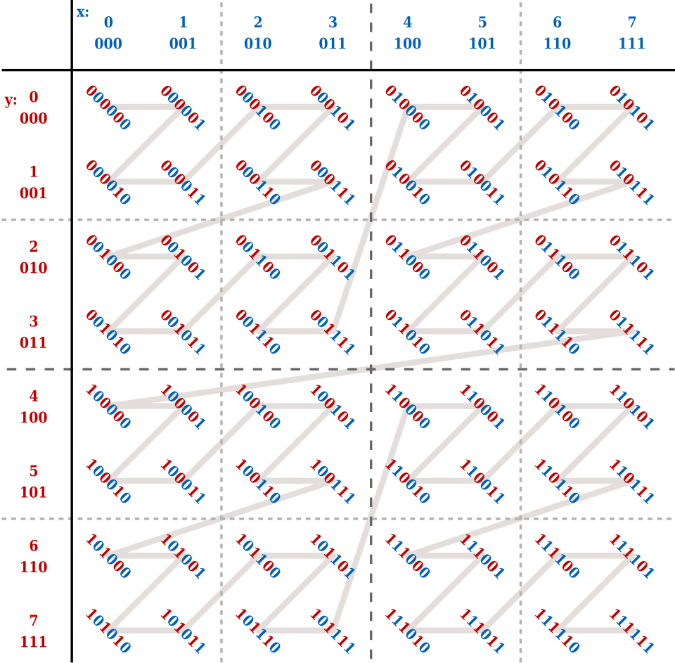
It can be used to find close values in multi-dimensional space.
Let's assume that we are finding values that belong to the given ranges 2<=x<=3 and 2<=y<=6. All values are closely located inside of the dotted rectangle: [12, 15] and [36, 45]. Note that there are some unwanted values in the middle of the ranges.

That's where BIGMIN and LITMAX come in. One of the limitations of Z-order curve is that values within a given range are not contiguous. Therefore, we need to find the minimum of larger range (BIGMIN) and the maximum of smaller range (LITMAX) to efficiently search for the desired values. For the details, please refer to the this paper: Multidimensional Range Search in Dynamically Balanced Trees.
Z-ordering in Delta Lake
So, how does it actually work in Delta Lake? Let's divide it into several phases.
Phase 1: Map arbitrary column values to discrete integers
In real world, column values are not integers. Therefore, it first quantizes values into integers. During this process, it simplifies values to a constant number of integers (numPartitions) by sampling data for each partition. That's the reason why it is not free from skew.
For example,
Values:    0    1    3   15   36   99
Range ID:  0    0    1    1    2    2  (with numPartitions=3)
Phase 2: Bit interleaving
After quantization, it computes bit interleaving with 32-bit integers. So, it has O(32 x N) complexity where N is the number of Z-ordering columns. For efficiency, it uses table lookup approach for small number of columns less than 8 to achieve O(4 x 8) complexity.
var bit = 31
while (bit >= 0) {
  var idx = 0
  while (idx < numCols) {
    ret_byte = (ret_byte | (((inputs(idx) >> bit) & 1) << ret_bit)).toByte
  }
}
Phase 3: Physical repartitioning
It redistributes according to the computed Z-values. Internally, it uses repartitionByRange which triggers:
- sampling data to determine range boundaries
- shuffling rows based on Z values
- creates
approxNumPartitionspartitions
File: skipping/MultiDimClustering.scala
var repartitionedDf = df.withColumn(repartitionKeyColName, mdcCol)
  .repartitionByRange(approxNumPartitions, col(repartitionKeyColName))
Phase 4: Intra-partition sorting
Finally, it sorts rows within each partition to maximize data locality.
File: skipping/MultiDimClustering.scala
if (sortWithinFiles) {
  repartitionedDf = repartitionedDf.sortWithinPartitions(repartitionKeyColName)
}
Usage of Z-ordering
You can trigger Z-ordering by executing
OPTIMIZE events WHERE date = '2021-11-18' ZORDER BY (eventType);WHERE clause is optional and should be Hive-style partition key columns.
Note that Z-ordering is not cheap; it requires a full table rewrite. Also, it is not idempotent which means that every time the Z-ordering is executed it will try to order entire partition again. So, well defined data management is key to maintain Z-ordered table.
So, carefully define partition key columns and Z-ordering columns. Here are some considerations:
When to choose Z-ordering columns:
- Is the column frequently used in predicates? If so, it is a good candidate for Z-ordering.
- Is the column a high cardinality column? Z-ordering is best fit for columns with high cardinality.
- Is the column a continuous value such as timestamps? It is best to use for range queries such as
BETWEENor>,<operators rather than exact equality.
When to choose partition key columns:
- If the table is frequently updated, consider using date or timestamp columns as partition key columns to avoid full table rewrite.