Deep dive into Delta Lake Liquid Clustering

In a previous article, we covered Z-ordering, an optimization technique for improving query performance in Delta Lake. But if you visit the Delta Lake documentation, you'll find recommendations like:

We recommend using liquid clustering

throughout their documentation. But why? What makes it better than Z-ordering and how does it work differently? In this article, we'll delve into Liquid Clustering.

This article is the second in Delta Lake deep dive series.

1. Deep dive into Delta Lake merge
2. Deep dive into Delta Lake Z-ordering
3. Deep dive into Delta Lake Liquid Clustering (this article)

Limitation of Z-ordering

Let's start with WHY it is proposed.

Z-ordering with Hive-style partitioning has two major limitations:

1. Once a table is partitioned, they cannot be changed
2. Z-ordering rewrites all data in the partition and cannot be done incrementally - they are NOT idempotent

The first two limitations make Z-ordering inflexible. It is crucial because query patterns evolve as business needs change, and the data structure must adapt accordingly.

So, liquid clustering was originally designed to address these limitations.

Hilbert curves

The design document for liquid clustering aims to improve upon Z-ordering's locality preservation using the Hilbert curve, a space-filling curve known to outperform Z-order curves.

Like Z-order curves, Hilbert curves map multidimensional points to a 1D sequence while preserving locality—points close in space remain close in the sequence. The key difference is that Hilbert curves achieve better locality with fewer "jumps" between distant points.

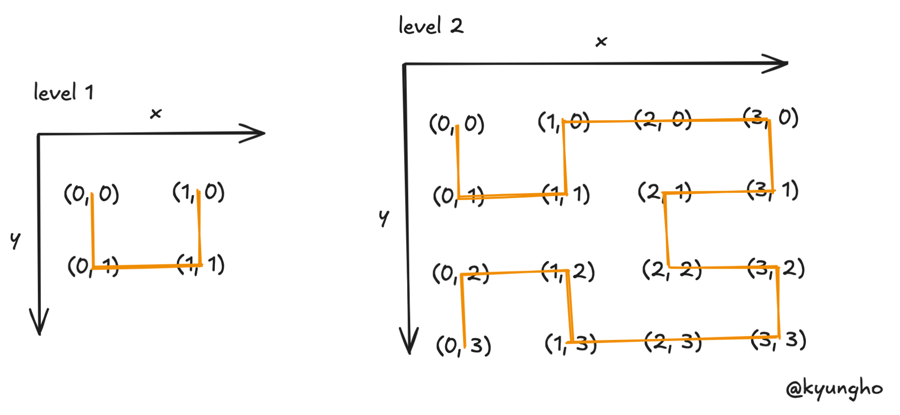
The simplest Hilbert curve is a U shape connecting 4 points in a 2x2 grid: (0,0) → (0,1) → (1,1) → (1,0).

At level 2, the curve divides a 4x4 grid into 4 quadrants, placing a smaller U shape in each. The bottom quadrants are rotated to maintain a continuous path, connecting all 16 points without jumps.

This recursive construction—divide, place, rotate, connect—extends to any level and any number of dimensions.

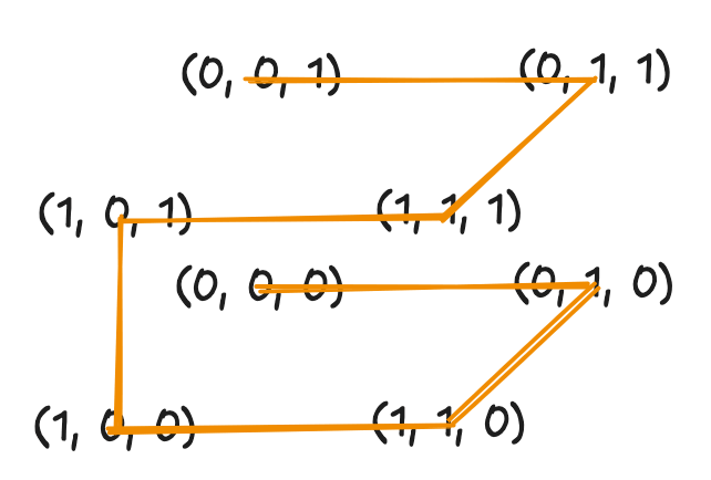
In 3D, the base shape becomes a path through 8 corners of a cube. Each level subdivides into 8 sub-cubes, with rotations ensuring continuity. Delta Lake uses this property to cluster data across multiple columns.

Why is Hilbert better than Z-order?

The diagram below compares both curves on an 8x8 grid. Numbers indicate the position in each curve's sequence.

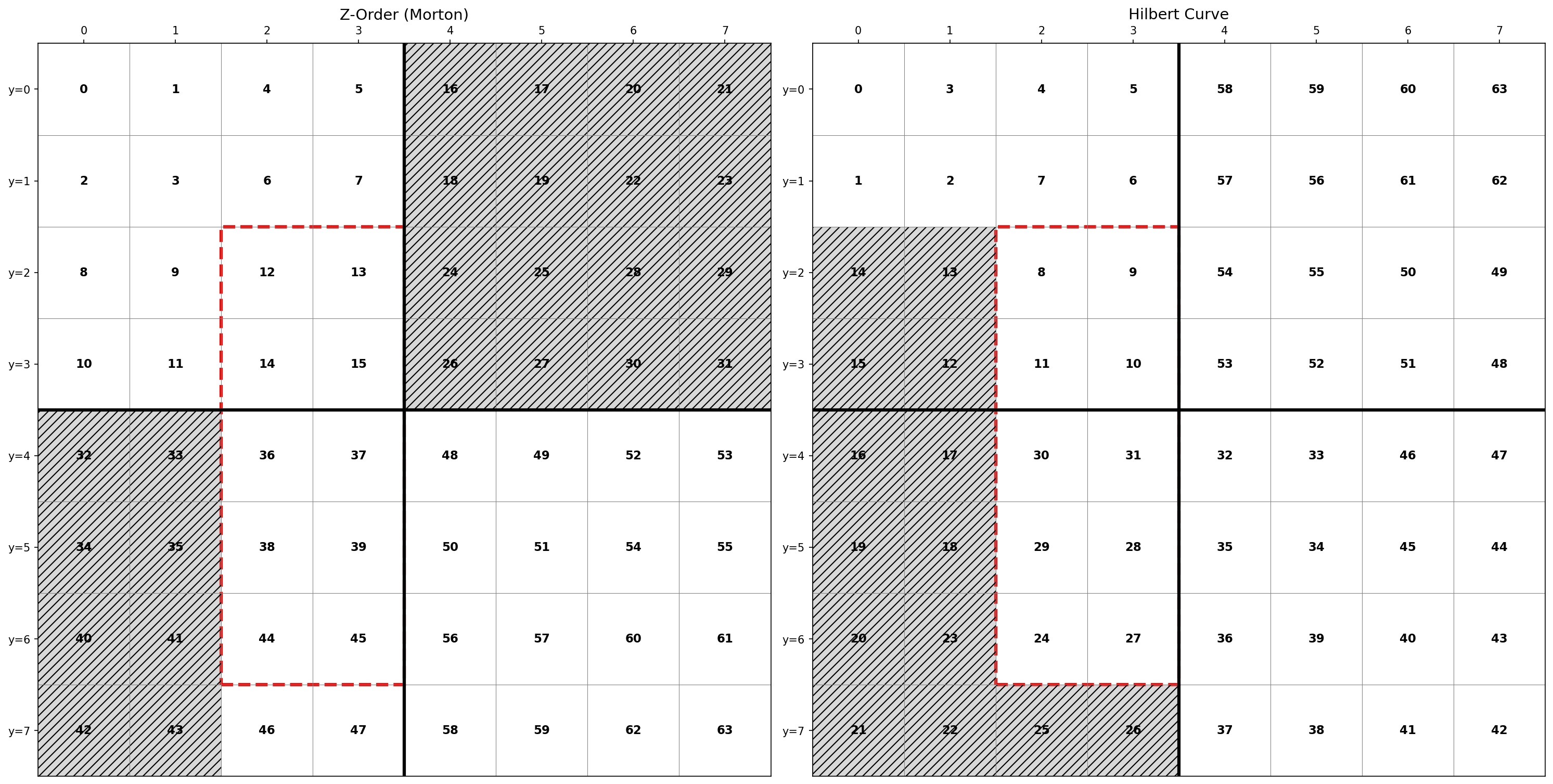
Consider a query filtering x=[2,3] and y=[2,6]—a rectangular region containing 10 points.

With Z-ordering, these points span indices 12 to 45. To find all matching data, Delta Lake must scan files covering this entire range of 34 index values, even though only 10 are relevant. That's 24 files scanned unnecessarily.

With Hilbert curves, the same 10 points span indices 8 to 31—a range of 24 values. Only 14 unnecessary files are scanned, a 42% reduction in wasted I/O.

This happens because Z-order curves have discontinuities where the path "jumps" across the grid, breaking locality. Hilbert curves maintain a continuous path, keeping nearby points in contiguous index ranges. For Delta Lake, contiguous ranges mean fewer files to scan and faster query execution.

Incremental clustering

Delta Lake introduces a concept of ZCubes, which is a group of files produced by the same OPTIMIZE job. Each ZCube has unique ZCUBE ID so that Delta Lake can distinguish fresh and unoptimized ZCubes.

ZCubes smaller than MIN_CUBE_SIZE are considered partial ZCubes. New data goes into partial ZCubes. OPTIMIZE then rewrites only these partial ZCubes rather than the entire table.

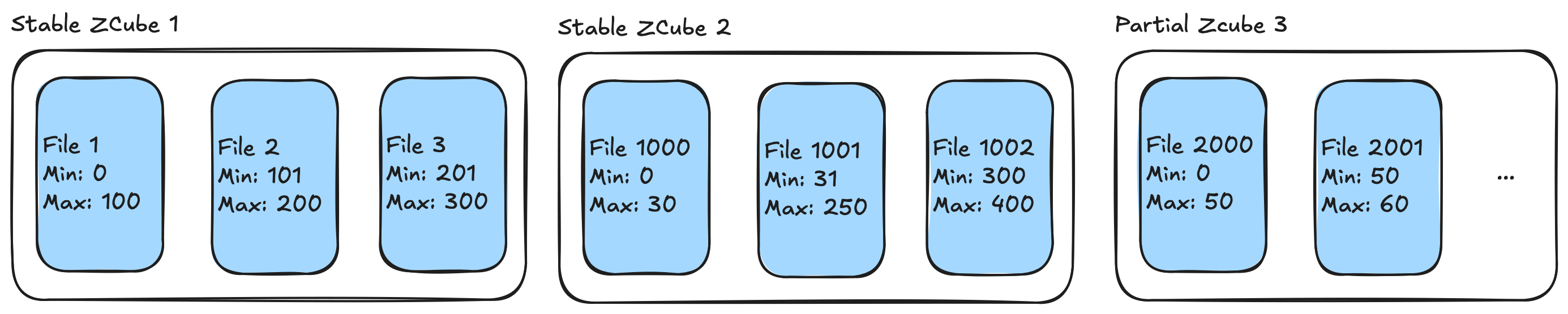
Stable ZCubes can become partial if DML deletes a significant portion of files.

One special case is when user changes clustering columns. This preserves stable ZCubes unchanged. New clustering applies only to data added after the change.

Liquid Clustering in Delta Lake

Liquid clustering is an advanced data organization technique in Delta Lake that addresses some of the limitations of Z-ordering.

Enable clustering when creating a table:

CREATE TABLE table1(col0 int, col1 string) USING DELTA CLUSTER BY (col0);

Change clustering columns on an existing table:

ALTER TABLE <table_name>
CLUSTER BY (<clustering_columns>)

Trigger clustering (incremental by default, or full rewrite):

OPTIMIZE <table_name>;
OPTIMIZE <table_name> FULL;

Inspect clustering configuration:

DESCRIBE DETAIL table_name;

Liquid Clustering Deep Dive

When OPTIMIZE runs on a clustered table, Delta Lake applies Hilbert clustering in four steps:

1. Quantization - Convert column values to discrete integer range IDs.
2. Hilbert index computation - Map N-dimensional points to 1D Hilbert indices.
3. Repartitioning by range - Physically redistribute rows based on Hilbert indices.
4. Sorting within partitions - Order rows by Hilbert index inside each partition.

Phase 1: Quantization

Hilbert curves operate on integer coordinates, but real data contains strings, timestamps, and decimals. Quantization bridges this gap by mapping any value to an integer range ID.

Delta Lake samples the data to find evenly-distributed boundaries, then assigns each value to a bucket. Values that are close together get the same or adjacent range IDs.

Values:    0    1    3   15   36   99
Range ID:  0    0    1    1    2    2  (with numPartitions=3)

Phase 2: Hilbert index computation

After quantization, each row has N integer coordinates (one per clustering column). The Hilbert algorithm converts these N coordinates into a single Long value—the row's position along the Hilbert curve.

The algorithm uses a state machine that walks the curve level by level. At each level, it looks at one bit from each coordinate, transforms it based on the current state (which tracks the curve's orientation), and accumulates the result.

File: HilbertIndex.scala

def translateNPointToDKey(point: Array[Int], k: Int): Long = {
  var result = 0L
  var currentState = 0

  // Walk the curve level by level
  while (i < k) {
    // Combine one bit from each dimension
    var z = 0
    while (j < n) {
      z = (z << 1) | ((point(j) >> (k - 1 - i)) & 1)
    }

    // Transform through state machine (handles curve rotations)
    val (h, nextState) = transform(z, currentState)
    result = (result << n) | h
    currentState = nextState
  }
  result
}

Phase 3: Repartitioning

Now every row has a Hilbert index. The next step groups rows with similar indices into the same partitions—which will become the same output files.

Delta Lake uses repartitionByRange rather than regular hash partitioning. Range partitioning samples the data to find boundaries that create balanced partitions, then shuffles rows so that adjacent Hilbert indices land in the same partition.

File: MultiDimClustering.scala

var repartitionedDf = df.withColumn(repartitionKeyColName, mdcCol)
  .repartitionByRange(approxNumPartitions, col(repartitionKeyColName))

Phase 4: Sorting within partitions

Finally, Delta Lake sorts rows within each partition by their Hilbert index. This arranges similar rows adjacent to each other in the output files.

File: MultiDimClustering.scala

if (sortWithinFiles) {
  repartitionedDf = repartitionedDf.sortWithinPartitions(repartitionKeyColName)
}

Caveats

• Delta Lake only supports up to 4 clustering columns for liquid clustering.
• Use high cardinality columns for better data skipping.
• If two columns are correlated, include only one.

Further Reading

• Liquid Clustering - Design Doc
• Liquid Clustering - Delta Lake
• Hilbert Curve - Wikipedia
• How Delta Lake Liquid Clustering conceptually works
• Comprehensive Guide to Databricks Optimization: Z-Order, Data Compaction, and Liquid Clustering